텐서플로 시작하기(Getting Started With TensorFlow)(3) tf.train tf.estimator API

출처 : https://www.tensorflow.org/get_started/get_started

이글은 영어 원본을 읽고 공부하면서 불필요한 내용 빼고 이해하기 쉽도록 적절히 내맘대로 작성해보았습니다. 이해가 잘못되어 원저자의 의도대로 번역이 안되어 있을 수도 있습니다. 이점 참고해서 읽어 주시면 고맙겠습니다

앞서 작성한 글

텐서플로 시작하기 (Getting Started With TensorFlow)(1) 

텐서플로 시작하기 (Getting Started With TensorFlow)(2) 

이 글은 앞서 작성한 글에 이어지는 글입니다.

tf.train API

TensorFlow는 손실 함수를 최소화하기 위해 각 변수를 천천히 변경하는 optimizers를 제공합니다. 가장 간단한  optimizers는 gradient descent(경사 하강법)입니다. 그것은 매개변수로 된 함수가 주어지면 함수의 값이 최소화되는 방향으로 매개변수를 변경하는 것을 반복적으로 수행하는 방법입니다. TensorFlow는 tf.gradients 함수를 사용하여 자동으로 생성 할 수 있습니다. 기울기를 계산해야 하므로 오차 함수는 미분 가능해야 합니다.  아래와 같이 사용합니다.

optimizer = tf.train.GradientDescentOptimizer(0.01)
train = optimizer.minimize(loss)

sess.run(init) # reset values to incorrect defaults.
for i in range(1000):
  sess.run(train, {x: [1, 2, 3, 4], y: [0, -1, -2, -3]})
print(sess.run([W, b]))

마지막 모델의 결과는 아래와 같이 나옵니다.

[array([-0.9999969], dtype=float32), array([ 0.99999082], dtype=float32)]

이 간단한 선형 회귀 모델이 TensorFlow 핵심 코드를 많이 필요로하지는 않지만 모델에 데이터를 입력하는 더 복잡한 모델과 방법은 더 많은 코드가 필요합니다. 따라서 TensorFlow는 일반적인 패턴, 구조 및 기능에 대해 더 높은 수준의 추상화를 제공합니다.

Complete program

완성 된 학습 가능한 선형 회귀 모델은 다음과 같습니다.

import tensorflow as tf
# Model parameters
W = tf.Variable([.3], dtype=tf.float32)
b = tf.Variable([-.3], dtype=tf.float32)
# Model input and output
x = tf.placeholder(tf.float32)
linear_model = W*x + b
y = tf.placeholder(tf.float32)
# loss
loss = tf.reduce_sum(tf.square(linear_model - y)) # sum of the squares
# optimizer
optimizer = tf.train.GradientDescentOptimizer(0.01)
train = optimizer.minimize(loss)
# training data
x_train = [1, 2, 3, 4]
y_train = [0, -1, -2, -3]
# training loop
init = tf.global_variables_initializer()
sess = tf.Session()
sess.run(init) # reset values to wrong
for i in range(1000):
  sess.run(train, {x: x_train, y: y_train})
# evaluate training accuracy
curr_W, curr_b, curr_loss = sess.run([W, b, loss], {x: x_train, y: y_train})
print("W: %s b: %s loss: %s"%(curr_W, curr_b, curr_loss))

실행 결과는 아래와 같습니다.

W: [-0.9999969] b: [ 0.99999082] loss: 5.69997e-11

loss는 아주 작은 숫자입니다 (거의 0에 가깝습니다). 이 프로그램을 직접 실행해보면 loss값과 일치하지 않습니다. 그 이유는 의사 난수 값으로 초기화되기 때문입니다.

그리고 이것을 TensorBoard 에서 시각화 해보면 아래와 같습니다.




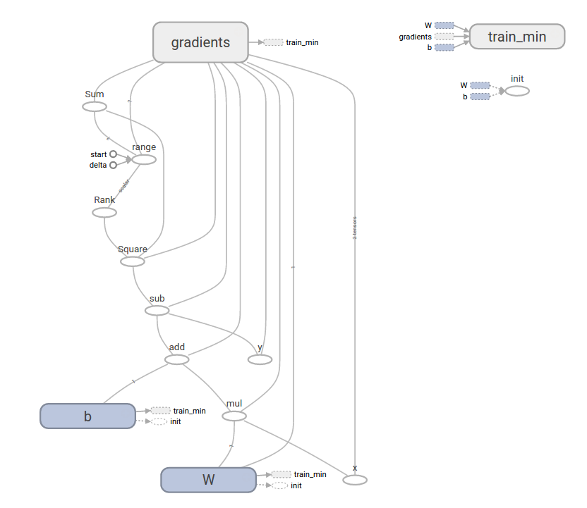
물론 이렇게 그대로 하면 시각화가 되지 않습니다.
시각화 예제는 아래 소스 참고 하시기 바랍니다.

TensorBoard 포함

import tensorflow as tf
# Model parameters
W = tf.Variable([.3], dtype=tf.float32)
b = tf.Variable([-.3], dtype=tf.float32)
# Model input and output
x = tf.placeholder(tf.float32)
linear_model = W*x + b
y = tf.placeholder(tf.float32)
# loss
loss = tf.reduce_sum(tf.square(linear_model - y)) # sum of the squares
# optimizer
optimizer = tf.train.GradientDescentOptimizer(0.01)
train = optimizer.minimize(loss)
# training data
x_train = [1, 2, 3, 4]
y_train = [0, -1, -2, -3]
# training loop
init = tf.global_variables_initializer()
sess = tf.Session()
file_writer = tf.summary.FileWriter('E:/work/ai/anaconda', sess.graph)
sess.run(init) # reset values to wrong
for i in range(1000):
  sess.run(train, {x: x_train, y: y_train})
# evaluate training accuracy
curr_W, curr_b, curr_loss = sess.run([W, b, loss], {x: x_train, y: y_train})
print("W: %s b: %s loss: %s"%(curr_W, curr_b, curr_loss))
file_writer.add_graph(sess.graph)
file_writer.close()

코드 분석

앞서 최소 값이 되기위하여 엑셀표를 참고하면 W,b가 어떤값일때 loss값이 최소가 되는지 살펴보아서 알고는 있습니다. 그러나 여기에서는 목표값을 모른다고 가정하고 train을 하게됩니다. train시 for i in range(1000): 에 의해서 1000번 train을 하면서 W,b 값을 변경하게 됩니다.
위 코드를 이해하기 위해서는 아래와 같이 소스를 변경해서 실행해보면 이해하기 쉽습니다.

train 변경

1 2 3 4 5 6 7 8 9 10 11 12 13 14 15 16 17 18 19 20 21 22 23 24 25 26 27 28 29 30 31 32 33 34 35 36 37 38 39 40 41

import tensorflow as tf # Model parameters W = tf.Variable([.3], dtype=tf.float32) b = tf.Variable([-.3], dtype=tf.float32) # Model input and output x = tf.placeholder(tf.float32) linear_model = W*x + b y = tf.placeholder(tf.float32) # loss loss = tf.reduce_sum(tf.square(linear_model - y)) # sum of the squares # optimizer optimizer = tf.train.GradientDescentOptimizer(0.01) train = optimizer.minimize(loss) # training data x_train = [1, 2, 3, 4] y_train = [0, -1, -2, -3] # training loop init = tf.global_variables_initializer() sess = tf.Session() sess.run(init) # reset values to wrong #for i in range(1000): # sess.run(train, {x: x_train, y: y_train}) curr_W, curr_b, curr_loss = sess.run([W, b, loss], {x: x_train, y: y_train}) print("W: %s b: %s loss: %s"%(curr_W, curr_b, curr_loss)) sess.run(train, {x: x_train, y: y_train}) curr_W, curr_b, curr_loss = sess.run([W, b, loss], {x: x_train, y: y_train}) print("W: %s b: %s loss: %s"%(curr_W, curr_b, curr_loss)) sess.run(train, {x: x_train, y: y_train}) curr_W, curr_b, curr_loss = sess.run([W, b, loss], {x: x_train, y: y_train}) print("W: %s b: %s loss: %s"%(curr_W, curr_b, curr_loss)) sess.run(train, {x: x_train, y: y_train}) curr_W, curr_b, curr_loss = sess.run([W, b, loss], {x: x_train, y: y_train}) print("W: %s b: %s loss: %s"%(curr_W, curr_b, curr_loss)) sess.run(train, {x: x_train, y: y_train}) curr_W, curr_b, curr_loss = sess.run([W, b, loss], {x: x_train, y: y_train}) print("W: %s b: %s loss: %s"%(curr_W, curr_b, curr_loss))

line 21,22 을 삭제하고 line 27,31,35,39에서 train을 한번씩 하도록 변경하고 train을 한 후 값을 출력할 수 있도록 변경하였습니다.

결과

(E:\Users\xxx\Anaconda3) E:\work\ai\anaconda>python tensor2.py
2017-11-19 22:19:07.041552: I C:\tf_jenkins\home\workspace\rel-win\M\windows\PY\36\tensorflow\core\platform\cpu_feature_guard.cc:137] Your CPU supports instructions that this TensorFlow binary was not compiled to use: AVX AVX2
W: [ 0.30000001] b: [-0.30000001] loss: 23.66
W: [-0.21999997] b: [-0.456] loss: 4.01814
W: [-0.39679998] b: [-0.49552] loss: 1.81987
W: [-0.45961601] b: [-0.4965184] loss: 1.54482
W: [-0.48454273] b: [-0.48487374] loss: 1.48251

결과를 살펴보면 loss값이 점차 줄어드는것을 볼 수 있습니다. 또한 아래 결과는 GradientDescentOptimizer인자값을 변경하면서 결과를 살펴보았습니다. 값이 작게되면 loss값의 변화가 작게되며, 값이 어느 정도 커지면 loss값이 늘어나게 되는 경우도 발생하게 됩니다. 이런 경우 루프를 아무리 많이 돌아도 loss값이 줄어들지 않게 됩니다. 따라서 적절한 값의 설정이 필요하며, 너무 작으면 loss를 줄이는데 굉장히 많은 loop가 필요하기 때문에 많은 시간을 필요로 합니다.

tf.train.GradientDescentOptimizer(0.001) 일때

W: [ 0.30000001] b: [-0.30000001] loss: 23.66
W: [ 0.24800001] b: [-0.31560001] loss: 20.811
W: [ 0.19943202] b: [-0.33003521] loss: 18.3294
W: [ 0.1540668] b: [-0.34338358] loss: 16.1677
W: [ 0.11169046] b: [-0.35571784] loss: 14.2848

tf.train.GradientDescentOptimizer(0.1) 일때

W: [ 0.30000001] b: [-0.30000001] loss: 23.66
W: [-4.9000001] b: [-1.8599999] loss: 712.098
W: [ 24.22000122] b: [ 8.22800064] loss: 22936.2
W: [-141.55599976] b: [-47.99440002] loss: 740011.0
W: [ 799.76879883] b: [ 272.31311035] loss: 2.38765e+07

tf.estimator

tf.estimator는 기계 학습의 메커니즘을 단순화하는 상위 수준의 TensorFlow 라이브러리입니다. 아래 내용을 포함합니다.
-훈련 루프 실행
-평가 루프 실행
-데이터 세트 관리
tf.estimator는 많은 공통 모델을 정의합니다.(여기서 모델이라고 하면, 선형회귀 같은것을 의미합니다.)
좀더 자세한 내용을 원하면 아래 주제를 더 살펴 봐도 됩니다.
https://www.tensorflow.org/programmers_guide/estimators
https://www.tensorflow.org/get_started/estimator
하지면 여기에서는 원본내용에서도 간단하게되어 있어 여기까지만 설명하도록 하겠습니다.

기본적인 용법

tf.estimator를 사용하면 선형 회귀 프로그램이 얼마나 단순해지는지 보여집니다.

# NumPy is often used to load, manipulate and preprocess data.
import numpy as npimport tensorflow as tf
# Declare list of features. We only have one numeric feature. There are many
# other types of columns that are more complicated and useful.
feature_columns = [tf.feature_column.numeric_column("x", shape=[1])]
# An estimator is the front end to invoke training (fitting) and evaluation
# (inference). There are many predefined types like linear regression,
# linear classification, and many neural network classifiers and regressors.
# The following code provides an estimator that does linear regression.
estimator = tf.estimator.LinearRegressor(feature_columns=feature_columns)
# TensorFlow provides many helper methods to read and set up data sets.
# Here we use two data sets: one for training and one for evaluation
# We have to tell the function how many batches
# of data (num_epochs) we want and how big each batch should be.
x_train = np.array([1., 2., 3., 4.])
y_train = np.array([0., -1., -2., -3.])
x_eval = np.array([2., 5., 8., 1.])
y_eval = np.array([-1.01, -4.1, -7, 0.])
input_fn = tf.estimator.inputs.numpy_input_fn(
    {"x": x_train}, y_train, batch_size=4, num_epochs=None, shuffle=True)
train_input_fn = tf.estimator.inputs.numpy_input_fn(
    {"x": x_train}, y_train, batch_size=4, num_epochs=1000, shuffle=False)
eval_input_fn = tf.estimator.inputs.numpy_input_fn(
    {"x": x_eval}, y_eval, batch_size=4, num_epochs=1000, shuffle=False)
# We can invoke 1000 training steps by invoking the  method and passing the
# training data set.
estimator.train(input_fn=input_fn, steps=1000)
# Here we evaluate how well our model did.
train_metrics = estimator.evaluate(input_fn=train_input_fn)
eval_metrics = estimator.evaluate(input_fn=eval_input_fn)
print("train metrics: %r"% train_metrics)
print("eval metrics: %r"% eval_metrics)

실행시키면 아래와 같은 결과가 나옵니다.

train metrics: {'average_loss': 1.4833182e-08, 'global_step': 1000, 'loss': 5.9332727e-08}
eval metrics: {'average_loss': 0.0025353201, 'global_step': 1000, 'loss': 0.01014128}

결과에서 eval loss 데이터를 보면 평가값이 높긴하지만 0에 가까운것을 보면 제대로 train되었다는것을 알 수 있습니다. (train 후 eval 을 하게되는데, 보통 train data와 다른값을 사용하여 eval을 하기 때문에 loss 값은 많이 차이 날 수 있습니다.)

A custom model

tf.estimator는 미리 준비된 모델만 이용할 수 있는건 아니고 직접 저수준 함수를 이용해서 커스텀 모델을 만들 수 있습니다. 여기 예제에서는 앞서 사용한 1차원 선형 회귀 모델을 커스텀 모델로 변경하였습니다. 앞서 tf.estimator.LinearRegressor 이것을 이용하는 부분이  model_fn을 만들고 tf.estimator.Estimator(model_fn=model_fn) 에 전달하는 부분이 다릅니다.

import numpy as npimport tensorflow as tf
# Declare list of features, we only have one real-valued feature
def model_fn(features, labels, mode):
  # Build a linear model and predict values
  W = tf.get_variable("W", [1], dtype=tf.float64)
  b = tf.get_variable("b", [1], dtype=tf.float64)
  y = W*features['x'] + b
  # Loss sub-graph
  loss = tf.reduce_sum(tf.square(y - labels))
  # Training sub-graph
  global_step = tf.train.get_global_step()
  optimizer = tf.train.GradientDescentOptimizer(0.01)
  train = tf.group(optimizer.minimize(loss),
                   tf.assign_add(global_step, 1))
  # EstimatorSpec connects subgraphs we built to the
  # appropriate functionality.
  return tf.estimator.EstimatorSpec(
      mode=mode,
      predictions=y,
      loss=loss,
      train_op=train)

estimator = tf.estimator.Estimator(model_fn=model_fn)
# define our data sets
x_train = np.array([1., 2., 3., 4.])
y_train = np.array([0., -1., -2., -3.])
x_eval = np.array([2., 5., 8., 1.])
y_eval = np.array([-1.01, -4.1, -7., 0.])
input_fn = tf.estimator.inputs.numpy_input_fn(
    {"x": x_train}, y_train, batch_size=4, num_epochs=None, shuffle=True)
train_input_fn = tf.estimator.inputs.numpy_input_fn(
    {"x": x_train}, y_train, batch_size=4, num_epochs=1000, shuffle=False)
eval_input_fn = tf.estimator.inputs.numpy_input_fn(
    {"x": x_eval}, y_eval, batch_size=4, num_epochs=1000, shuffle=False)
# train
estimator.train(input_fn=input_fn, steps=1000)
# Here we evaluate how well our model did.
train_metrics = estimator.evaluate(input_fn=train_input_fn)
eval_metrics = estimator.evaluate(input_fn=eval_input_fn)
print("train metrics: %r"% train_metrics)
print("eval metrics: %r"% eval_metrics)

결과는 이전과 크게 다르지 않습니다.

train metrics: {'loss': 1.227995e-11, 'global_step': 1000}
eval metrics: {'loss': 0.01010036, 'global_step': 1000}