Neural Networks
이번에는 아래 링크를 공부해 보도록 하겠습니다.
https://pytorch.org/tutorials/beginner/blitz/neural_networks_tutorial.html
PyTorch에서 Neural Networks는 torch.nn 패키지를 이용해서 구성되어질 수 있습니다.
nn.Module에는 레이어와 출력을 반환하는 메서드 forward(input)이 포함되어 있습니다. (아래 Define the network 예제를 살펴보면, 네트워크를 만들때 class Net(nn.Module): , def forward(self, x): 메소드가 존재해야한다는 의미이고 해당 메소드의 리턴값이 output이 된다는 의미입니다. )
이미지 분류의 예를 보면 아래와 같습니다.
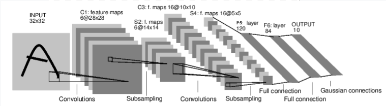
https://pytorch.org/tutorials/_images/mnist.png
이것은 단순한 feed-forward network 입니다. input을 가져가고 입력은 뒤쪽 다른 layer의 또 다른 입력이 됩니다. 결국 마지막에는 출력이 주어집니다.
전형적인 neural network을 위한 훈련(training)은 아래 절차는 따릅니다.
- 약간의 learnable 인자들 (or weights 가중치 값)을 가지는 neural network를 정의 합니다.
- 입력 데이터셋 전체를 반복합니다.
- network를 통한 입력 처리
- loss(손실) 계산 (출력이 옳은 값과 얼마나 떨어져 있는지)
- 네트워크의 인자 이용 그라디언트 역전파
- 네트워크의 가중치 업데이트, 단순 업데이트 룰 사용 : weight = weight - learning_rate * gradient
Define the network(네트워크 정의)
기본적인 network 구성한 예제입니다.
아래예에서 nn.Conv2d, nn.Linear, F.max_pool2d, F.relu 들은 PyTorch에 미리 준비된 고수준 레벨의 함수입니다. 아래 링크를 참고하면 됩니다.
https://pytorch.org/docs/stable/nn.html#torch.nn.Conv2d
https://pytorch.org/docs/stable/nn.html#torch.nn.Linear
https://pytorch.org/docs/stable/nn.html#torch.nn.functional.max_pool2d
https://pytorch.org/docs/stable/nn.html#torch.nn.functional.relu
import torch
import torch.nn as nn
import torch.nn.functional as F


class Net(nn.Module):

    def __init__(self):
        super(Net, self).__init__()
        # 1 input image channel, 6 output channels, 5x5 square convolution
        # kernel
        self.conv1 = nn.Conv2d(1, 6, 5)
        self.conv2 = nn.Conv2d(6, 16, 5)
        # an affine operation: y = Wx + b
        self.fc1 = nn.Linear(16 * 5 * 5, 120)
        self.fc2 = nn.Linear(120, 84)
        self.fc3 = nn.Linear(84, 10)

    def forward(self, x):
        # Max pooling over a (2, 2) window
        x = F.max_pool2d(F.relu(self.conv1(x)), (2, 2))
        # If the size is a square you can only specify a single number
        x = F.max_pool2d(F.relu(self.conv2(x)), 2)
        x = x.view(-1, self.num_flat_features(x))
        x = F.relu(self.fc1(x))
        x = F.relu(self.fc2(x))
        x = self.fc3(x)
        return x

    def num_flat_features(self, x):
        size = x.size()[1:]  # all dimensions except the batch dimension
        num_features = 1
        for s in size:
            num_features *= s
        return num_features


net = Net()
print(net)
Out:
Net(
  (conv1): Conv2d(1, 6, kernel_size=(5, 5), stride=(1, 1))
  (conv2): Conv2d(6, 16, kernel_size=(5, 5), stride=(1, 1))
  (fc1): Linear(in_features=400, out_features=120, bias=True)
  (fc2): Linear(in_features=120, out_features=84, bias=True)
  (fc3): Linear(in_features=84, out_features=10, bias=True)
)
학습 가능한 매개 변수는 net.parameters()에 의해 반환됩니다.
params = list(net.parameters())
print(len(params))
print(params[0].size())  # conv1's .weight
Out:
10
torch.Size([6, 1, 5, 5])
참고 :이 네트(LeNet)에 대한 예상 입력 크기는 32x32입니다. 이 망을 MNIST 데이터 세트에 사용하려면 데이터 세트의 이미지를 32x32크기로 조정하세요
input = torch.randn(1, 1, 32, 32)
out = net(input)
print(out)
Out:
tensor([[-0.0184,  0.0634, -0.0269,  0.0710, -0.0038, -0.0464, -0.0063,
         -0.0751, -0.1399,  0.0892]])
랜덤 그라디언트를 가지고 backward를 수행합니다.
(왜 아래와 같은 동작이 필요한지는 잘모르겠습니다.)
net.zero_grad()
out.backward(torch.randn(1, 10))
Loss Function
손실 함수는 (출력, 대상) 입력 쌍을 사용하고 출력이 대상에서 얼마나 멀리 떨어져 있는지 추정하는 값을 계산합니다.
nn 패키지에는 여러 가지 손실 함수가 있습니다.
http://pytorch.org/docs/nn.html#loss-functions
간단한 손실은 다음과 같습니다. nn.MSELoss - 입력과 대상 간의 평균 제곱 오류를 계산합니다.
예)
output = net(input)
target = torch.arange(1, 11)  # a dummy target, for example
target = target.view(1, -1)  # make it the same shape as output
criterion = nn.MSELoss()

loss = criterion(output, target)
print(loss)
Out:
tensor(38.7042)
https://pytorch.org/docs/stable/torch.html?highlight=arange
target.view 참고 : 텐서의 차원을 변경한다. -1은 축이 자동으로 설정된다.
https://pytorch.org/docs/stable/tensors.html?highlight=view#torch.Tensor.view
import torch

target = torch.arange(1, 11)  # a dummy target, for example
print (target)
target = target.view(1, -1)  # make it the same shape as output
print (target)

(*** result ***)
(base) E:\pytorch>python test.py
tensor([  1.,   2.,   3.,   4.,   5.,   6.,   7.,   8.,   9.,  10.])
tensor([[  1.,   2.,   3.,   4.,   5.,   6.,   7.,   8.,   9.,  10.]])
제일 위의 out을 보면 아래와 같은 형태를 지니기 때문에
tensor([[-0.0184,  0.0634, -0.0269,  0.0710, -0.0038, -0.0464, -0.0063,
         -0.0751, -0.1399,  0.0892]])
view를 이용해 출력값을 아래와 같은 형태로 변경하였습니다.
tensor([[ 1., 2., 3., 4., 5., 6., 7., 8., 9., 10.]])왜냐하면 target이 옳은(목적) 값이라고 가정하기 때문입니다. 그리고 output과 target이 차이가 loss(손실)이 되기 때문에 같은 형태를 지닙니다.
.grad_fn 속성을 사용하여 역방향으로 손실을 추적하면 다음과 같은 계산 그래프가 표시됩니다.
input -> conv2d -> relu -> maxpool2d -> conv2d -> relu -> maxpool2d
      -> view -> linear -> relu -> linear -> relu -> linear
      -> MSELoss
      -> loss
따라서 loss.backward ()를 호출하면 전체 그래프가 손실에 대해 차등화(미분된)됩니다. 손실 및 requires_grad = True 인 그래프의 모든 텐서는 그라데이션으로 누적 된 .grad Tensor를 갖습니다.
예를 들어 몇 가지 단계를 backward 진행해 봅시다.
print(loss.grad_fn)  # MSELoss
print(loss.grad_fn.next_functions[0][0])  # Linear
print(loss.grad_fn.next_functions[0][0].next_functions[0][0])  # ReLU
Out:
<MseLossBackward object at 0x7f12da7f6710>
<AddmmBackward object at 0x7f12da7f6128>
<ExpandBackward object at 0x7f12da7f6128>
Backprop
오류를 back propagate(역전파) 하려면 loss.backward()를 사용해야합니다. 그래디언트가 기존 그라디언트에 누적되면 기존 그라디언트를 지워야합니다.
이제는 loss.backward ()를 호출하고 conv1의 뒤쪽 전후에 바이어스 그래디언트를 살펴 보겠습니다.
net.zero_grad()     # zeroes the gradient buffers of all parameters

print('conv1.bias.grad before backward')
print(net.conv1.bias.grad)

loss.backward()

print('conv1.bias.grad after backward')
print(net.conv1.bias.grad)
Out:
conv1.bias.grad before backward
tensor([ 0.,  0.,  0.,  0.,  0.,  0.])
conv1.bias.grad after backward
tensor(1.00000e-02 *
       [-4.6071, -2.4962,  1.5047, -4.6816, -3.6782, -5.3738])
Update the weights
실제로 사용되는 가장 단순한 업데이트 규칙은 확률 경사 하강법 입니다. Stochastic Gradient Descent (SGD)
weight = weight - learning_rate * gradient
간단한 파이썬 코드를 사용하여 구현할 수 있습니다. (아래 코드)
당신이 neural networks를 사용하면, 당신은 다양한 다른 업데이트 룰들을 (SGD, Nesterov-SGD, Adam, RMSProp 등등등) 사용 하기를 원합니다, 이것을 동작시키기 위해서 우리는 작은 패키지를 사용합니다. 이 모든 방법을 구현하는 torch.optim, 이것을 사용하는것은 매우 간단합니다.learning_rate = 0.01 for f in net.parameters(): f.data.sub_(f.grad.data * learning_rate)
import torch.optim as optim

# create your optimizer
optimizer = optim.SGD(net.parameters(), lr=0.01)

# in your training loop:
optimizer.zero_grad()   # zero the gradient buffers
output = net(input)
loss = criterion(output, target)
loss.backward()
optimizer.step()    # Does the update
이번에는 전체적으로 내용이 어렵습니다. 모르는 내용도 많고... , 좀 더 쉬우면서도 좋은 예제를 공부하도록 하겠습니다.
댓글 없음:
댓글 쓰기